FLake is freely available under the terms of the MIT license.
These files contain:
The forthcoming text presents a couple of hints that should help users to avoid the application of FLake beyond the limits of applicability of the model. Since FLake is a one-dimensional two-layer model, caution should be exercised in "extreme" cases, e.g. when FLake is applied to very shallow or very deep lakes. Some caution is also required when interpreting the model results.
In case a basin-mean temperature structure is a major concern, experience suggests that the best results (first of all, with respect to the lake surface temperature and to the ice cover) are obtained when a mean depth of a lake/reservoir in question is used, not its maximum depth or a depth at a particular location. This is actually consistent with a single-column nature of the model.
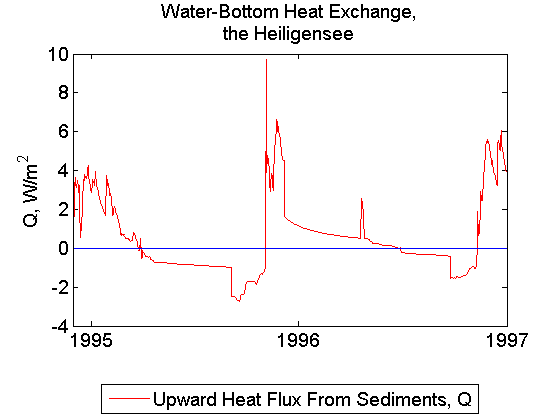
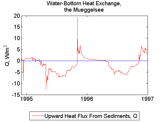
Thermal interaction between the water column and the bottom sediments is an issue for shallow lakes only. A seasonal cycle in shallow lakes may be noticeably affected by the accumulation of heat in the bottom sediments during spring and summer and the release of heat from the sediments during autumn and, in particular, winter. Apart from shallow lakes, the bottom heat flux can be set to zero. To do so, just set a logical switch lflk_botsed_use to .FALSE. in MODULE flake_configure (see the Synopsis of FLake Routines). Experience suggests that for lakes deeper than about 5 m the heat flux through the bottom can safely be neglected. In case the interaction between the water column and the bottom sediments is to be accounted for, prior empirical information is required to estimate the depth of the thermally active layer of bottom sediments, FLake variable depth_bs_lk , and the climatological-mean temperature at that depth, T_bs_lk . Unfortunately, such information is rarely available. As a rule of the thumb, an estimate in the range from about 4 m to about 10 m may be used for depth_bs_lk, and T_bs_lk may be set to a long-term (annual, decadal) mean of the water temperature near the lake bottom.
Strictly speaking, FLake is not suitable for deep lakes, where a two-layer representation of the temperature-depth curve with the lake thermocline extending from the outer edge of the upper mixed layer down to the lake bottom becomes inapplicable. For deep lakes, it is suggested to run FLake with a "false bottom". That is, an artificial lake bottom is set at a depth of about 50 m (perhaps 60 m), and the bottom-sediment module is switched off. The reasoning behind this trick is pretty simple. The deep abyssal zone of a temperate deep lake is usually filled with the water at the temperature close the temperature of maximum density, FLake variable tpl_T_r , and seasonal variations of abyssal temperature are usually small. Setting bottom heat flux to zero and using tpl_T_r as the initial condition for the water temperature at the bottom, one can expect FLake to reproduce this behaviour. Notice, however, that equatorial lakes may have their abyssal temperature well above tpl_T_r and they may never mix down to the bottom. In such a case, it is better to initiate FLake with the "climatological mean" temperature profile. Such profile can be obtained with FLake by computing a perpetual year solution.
Using the exponential approximation of the decay law for the flux of solar radiation, the optical characteristics of the lake water are given by the number of wavelength bands, the fractions of the total radiation flux for different wavelength bands, and the attenuation coefficients γ for different bands. The optical characteristics are lake-specific and should be estimated in every particular case. If empirical data are lacking, default values of the optical characteristics offered by FLake can be used (see the FLake source code for details). The simplest option is the one-band approximation with γ =3 m -1 that leads to the absorption of 95% of the incoming solar radiation within the uppermost 1 m of the lake water. For the lake ice, the recommended choice is the "opaque ice" one-band approximation with a very large value of γ =10 7 m -1 leading to the absorption of solar radiation at the ice surface.
Although provision is made to model the evolution of snow cover above the lake ice, the snow module of FLake has not been sufficiently tested so far. Any contribution along this line is very welcome! A recommended choice at the moment is to account for the effect of snow implicitly (parametrically) through the dependence of the ice surface albedo with respect to solar radiation on the surface temperature. To implement this choice, one only has to set the rate of snow accumulation to zero (see the Synopsis of FLake Routines for details). Make sure to specify the ice surface albedo in a rational way as e.g. in SUBROUTINE flake_interface .
The initialisation of FLake is straightforward if the integration is started when the lake considered is mixed down to the bottom and the ice is absent. Then, the model is initialised as follows (see SUBROUTINE flake_interface , variables h_snow_in, h_ice_in, T_snow_in, T_ice_in, C_T_in, T_mnw_in, T_wML_in, T_bot_in, T_B1_in, h_ML_in and H_B1_in ). The snow thickness and the ice thickness are set to zero, the surface temperatures of snow and of ice are (formally) set to the fresh-water freezing point, the shape factor with respect to the temperature profile in the thermocline is (formally) set to its minimum value of 0.5, and the mean temperature of the water column, the mixed-layer temperature and the bottom temperature are all set equal to the observed water temperature. If the bottom sediment module is switched off, the choice of initial values of the thickness of the upper layer of bottom sediments penetrated by thermal wave and of the temperature at that depth is irrelevant. In case the bottom sediment module is switched on, the observed values of the above two variables should be used. If no observational data are available, the thickness of the upper layer of bottom sediments is set to depth_bs_lk and the temperature at that depth is set to T_bs_lk , see (ii) above. In the event that the lake considered is initially stratified, some caution is required when setting FLake variables that specify the water temperature profile. That is, T_mnw, T_wML, T_bot, h_ML and C_T cannot be set completely independently as they are functionally related through the self-similar parameterisaton of the evolving temperature profile (see Eq. (23) in Mironov 2008). It is recommended to set the mean temperature of the water column, T_mnw , as close to its observed value as possible (this is important as T_mnw represents the heat content of a lake) and to adjust the other variables as needed so that Eq. (23) is satisfied. In the event of FLake initialisation during the period of ice cover, the initial values of ice thickness an of ice surface temperature should be set according to the observation. If the snow above the lake ice is not considered explicitly (a recommended choice), h_snow is set equal to zero and T_snow is (formally) set equal to T_ice .
A perpetual year solution represents the annual cycle of temperature and mixing in a given lake that corresponds to a given annual cycle of input meteorological quantities (temperature, humidity and wind speed in the surface air layer, downward radiation fluxes) that are used to force the lake model. Starting with arbitrary initial conditions, the year-long simulation is repeated, using one and the same annual cycle of forcing. The initial conditions for the next year-long run are specified using the values of the lake-model prognostic variables at the end of the previous year-long run. After a few model years, a periodic "perpetual year" solution is obtained. That is, running the model for one more year will not change the annual cycle of the lake-model variables. To obtain a perpetual year solution, FLake usually requires less than ten iterations (year-long runs) if a "reasonable" initial state is used that can be set on the basis of common sense. A perpetual year solution obtained with FLake is useful in many respects. For example, it may give an idea of the state of the lake in question if no data from measurements in the lake are available (but the atmospheric forcing can be specified in a rational way).
The windows-version of the FLake is compiled using Intel Fortran 8.1 for Windows under WinXP and should run on virtually any 32-bit Windows system. The main program in source files was slightly changed in comparison to the original Unix-version in order to provide a quick model reconfiguration without editing the source files.
Download .ZIPMETEOFILE variable (see examples in .nml files).
The file consists of 6 columns divided by space characters with following values (See example files Potsdam80-96.dat, and Stechlin94-98.dat from Test Runs):
| 1 | 2 | 3 | 4 | 5 | 6 |
|---|---|---|---|---|---|
| Sequential number | Solar Radiation (W/m2) | Air Temperature (oC) | Air Humidity (mb) | Wind Speed (m/s) | Cloudiness (0-1) |
TIME_STEP_NUMBER in the
namelist file.
Put all 3 files in the same directory, open the directory in the Windows Explorer and type in the command
line
(press "Windows key"+R to call the command window): flake < YOURFILE >, where <
YOURFILE >
is the name of Your namelist configuration file.
The file with modeling results will be created after a successful model run.
The output file name is that you have given in the namelist file as the value
for the OUTPUTFILE variable. Variables are in columns, variable names are given in the first
row. These
are:
If you use MATLAB for postprocessing and analysis of results the matlab-script ReadFlake.m can help importing data directly to MATLAB. Just run it from the matlab prompt.
Three long-term FLAKE calculations are presented below tested against observations data on vertical temperature structure. Three German lakes are simulated, the Heiligensee, the Mueggelsee and the Stechlinsee, located in the same climatic zone, but revealing esssentially different temperature and mixing regimes, mostly on account of different morphometry. This choice provides with opportunity of testing the model reliability for various mixing conditions. The model input and output files can be downloaded below and used for testing your copy of FLake and for further modification.
Test runs were performed in frames of research projects KI 853/2-1 and KI 853/3-1 funded by the German Science Foundation (DFG). Lake data collected at the Leibniz-Institute of Freshwater Ecology and Inland Fisheries, Berlin. Meteorological data are provided by the German Weather Service.
The model configuration is similar in all three cases and is typical for long-term simulations covering more than one year:
h_ML_in in the namelist files) is of no matter in this case. Otherwise, if you
start
the simulation in stratified conditions (e.g. in mid-Summer), an appropriate initial mixed layer depth
h_ML_in should be given among with the surface temperature T_wML_in
and the bottom temperature T_bot_in.
del_time_lk = 86400.0 [s]. Correspondingly,
the input meteorological data are daily averaged. By this, all diurnal variations
are filtered out. This averaging is consistent with horizontal spatial averaging over the lake
as soon as short-term processes with periods less than one day are usually include essential
spatial inhomogeneity (seiching, differential heating between near-shore areas and the deep part etc).
depth_bs_lk = 5.0 [m], T_bs_lk = 4.0 [oC].
You can switch the sediments layer off by choosing sediments_on = .FALSE. in the
&LAKE_PARAMS group of the namelist files.
extincoef_optic [m-1].
Water transparency conditions expressed by extincoef_optic differ for all three lakes
and contribute significantly to the vetical temperature structure. Thus, according to the model,
an increase in water transparency of the dimictic Heiligensee to
that of the polymictic Mueggelsee would also follow in occasional breakdown of the
summer thermocline, i.e. in transition to polymictic conditions. One can verify it by changing the value
of extincoef_optic in Heiligensee80-96.nml from
1.2
to 0.7-0.9 [m-1]
and running The Heiligensee test case.
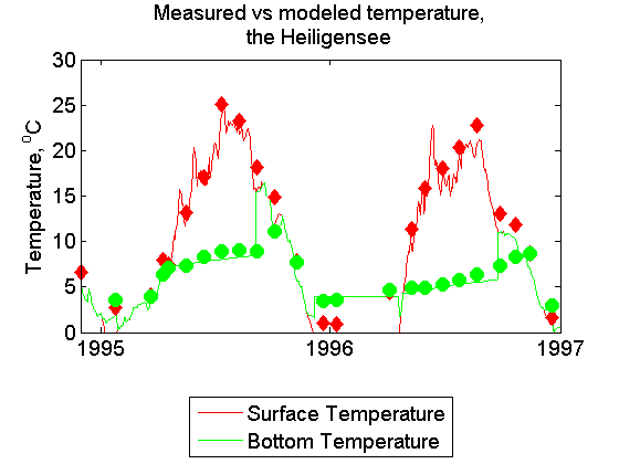
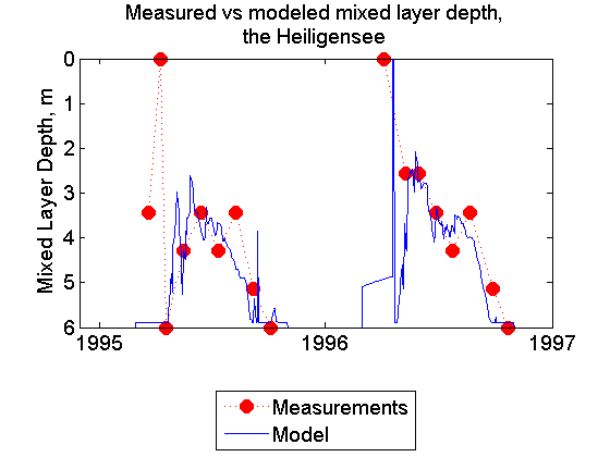
Shallow lake located in the north part of Berlin, Germany. mean depth 5.9m, maximum depth 8.1m, lake area 0.9km^2.
The lake is dimictic, i.e. is mixed down to the bottom twice a year in the spring and in the autumn. The lower part of the water column remains stratified duruing the summer, which behaviour is also predicted by the model.
To start the case on your computer:Heiligensee80-96.rslt should be identical to
the provided Heiligensee80-96.test
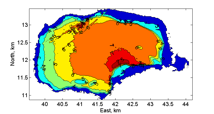
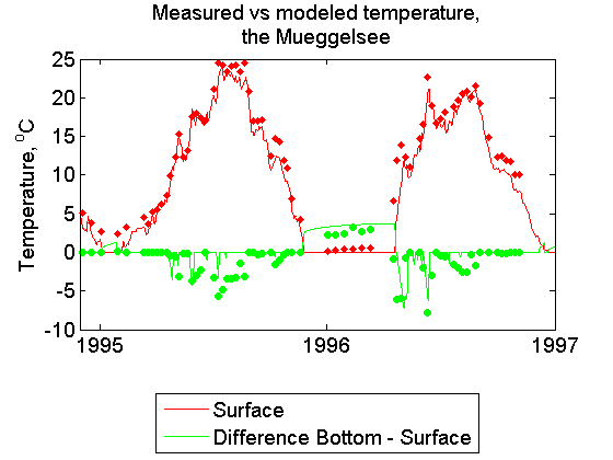
Shallow lake located in the south-east part of Berlin, Germany. mean depth 4.5m, maximum depth 8.0m, lake area 7.3 km^2.
The lake is polymictic, i.e. is mixed down to the bottom repeatedly during a year with occasional vertical stratification periods in summer. Therefore, no mixed layer depth is shown in figures, but the surface-bottom temperature difference. The same meteorology input is used here as for the Heiligensee because both lakes are situated close to each other.
To start the case on your computer:Mueggelsee80-96.rslt should be identical to
the provided Mueggelsee80-96.test
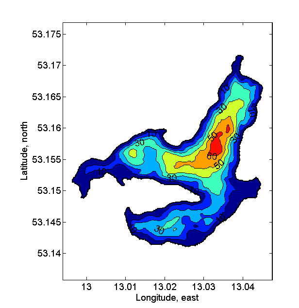
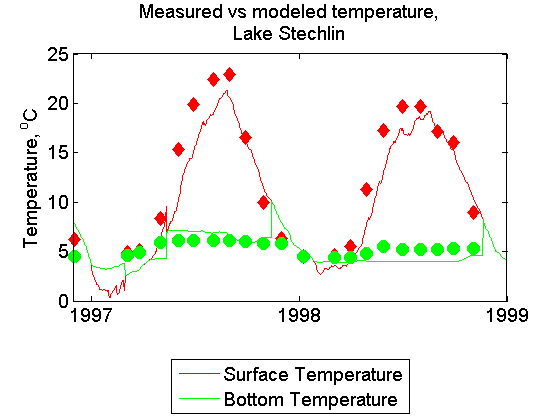
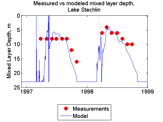
The lake is located 100km north to Berlin. mean depth 23.0m, maximum depth 68.0m, lake area 4.3km^2.
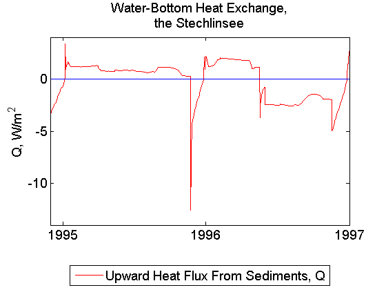
The lake can be classified as deep dimictic. A strong thermocline exists during summer at 5-10m depth, and near-bottom temperatures stay at 4-6^oC. Note the small heat exchange between water and sediments in the last figure. The meteorology input from the near-shore station is used.
To start the case on your computer: